1. Introduction
This note focus on the dynamic memory allocation. An typical application is the dynamic allocation of storage space to processes, which is a classic problem in operating systems. When a process arrives, it is assigned a contiguous storage area on the device. Once allocated, this area remains fixed since processes cannot be relocated. At an unknown future time, the process departs, freeing its allocated space for reuse. Over time, this cycle of allocation and deallocation creates unused gaps, or “holes”, within the storage device, leading to fragmentation.
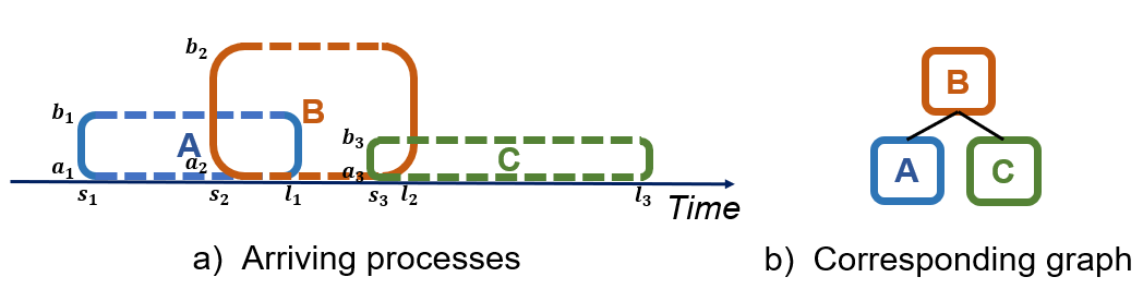 Figure 1: Dynamic memory allocation request from processes and corresponding graph.
The Dynamic Memory Allocation (DMA) problem is equivalent to graph coloring from problem on an undirected weighted graph $G=(V,E)$ defined as follows. Each vertex in $v_i\in V$ is an event with live range $[s_i,l_i]$ and weight $[a_i,b_i]$ ($a_i$ and $b_i$ are both integers and $b_i- a_i$ is the storage it need to allocate), two vertices are connected with an edge if and only if their live range are overlapped. A coloring on $G$ is a range-level coloring of each vertex, which means the color on interval vertex $v_i$ is a color range $[c_l,c_r]$. And a valid coloring on $G$ ensures that adjacent vertices have no overlapped color range.
Research on dynamic memory allocation (DMA) algorithms primarily focuses on two objectives:
minimizing allocation time [1] and reducing wasted memory space [2,3,4].
In this discussion, we focus on the latter—minimizing wasted space.
This goal is closely related to the equivalent graph coloring problem,
where the objective is to minimize the maximum upper bound of the color range.
Previous studies [5] have established that determining an optimal weighted coloring for such problems is NP-complete.
Numerous online algorithms have been developed to address the challenge of minimizing wasted space in DMA.
Among the most natural heuristics are First Fit and Best Fit.
Other strategies can be classified as segregated storage methods,
which partition memory into blocks of varying sizes and allocate memory to different types of requests from different types of blocks.
We will introduce several existing online algorithms for dynamic memory allocation (DMA) and conduct a competitive analysis of these algorithms.
2. First Fit
The First Fit approach allocates memory by locating the first available block that satisfies the requirements of the current process.
Robson [6] analysis the worst case of First Fit and bound the competitive ratio by $O(\log W_{max})$. Luby et al. [2] established a competitive ratio of $\Theta (\log k)$ for First Fit. Putting these all together, the competitive ratio of First Fit is $\min\lbrace\Theta (\log W_{max}),\Theta (\log k)\rbrace$. Here, $W_{max}$ is the maximum memory requested by a process and $k$ is the maximum number of active processes at the same time.
For simplicity, we assume the memory starts at address $0$. We also assume that the maximum sum of simultaneous processes allocation requirement is $w^{\star}$. Note that $OPT\ge w^{\star}$. Also note that in the graph we introduced in Section 1, $k$ is the maximum clique size and $w^{\star}$ is the maximum weight sum of all cliques.
2.1 Competitive Analysis for Ratio $\Theta (\log W_{max})$
The main ideas of the analysis is that occupied memory slice are scattered in the memory space, but the sum of their size should not exceed the maximum simultaneously allocated memory.
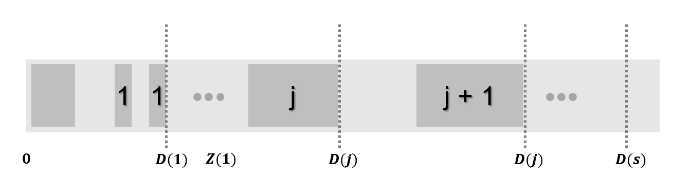 Figure 2: Demonstration of the memory layout at certain timestamp. We partition the memory space into different segments based on allocated space of different size and use this in our analysis.
Claim 1. Let $Z(i)=\frac{w^{\star}}{i \ln 2}$, all requests of size $j$ will be allocated before address $\sum_{i=1}^{j}Z(i)$.
Proof. We prove by induction. When $j=1$, $\sum_{i=1}^{j}Z(i)=Z(1)=\frac{w^{\star}}{\ln 2}>w^{\star}$. By the definition of $w^{\star}$, the request of size $1$ will be allocated before address $w^{\star}$. As a result, the claim holds for $j=1$.
Assume the claim holds for $j=s$, then for $j=s+1$, we prove the claim by contradiction. Define $D(j)$ as the actually used memory space to allocate memory to requests of size $j$. By definition, $D(j)\le \sum_{i=1}^{j}Z(i)$. Figure 2 gives demonstration of the memory layout with marked $D(j),Z(j)$. If there exists a request of size $s+1$ fail to be allocated before $\sum_{i=1}^{s+1}Z(i)$, we estimate the occupied memory space. The occupied memory can be classified as follows,
-
The area of occupied memory in segments with memory address $[0,D(1)], [D(1)+1,D(2)],\cdots , [D(s-1)+1,D(s)]$. Since $s+1$ fail to fit into any of the fragments in these segments, the fragments are at most $s$. Taking $D(0)=-1$, for each segments $[D(j)+1,D(j+1)]$, the occupied portion is at least $\frac{j+1}{j+s+1}$. So the occupied space before $D(s)$ is at least $S_1= \sum_{j=0}^{s-1}\frac{(D(j+1)-D(j))(j+1)}{j+s+1}$.
-
Now we consider the area before the highest address $s+1$ request can be allocated. For area between $[D(s)+1,\sum_{i=1}^{s+1}Z(i)-(s+1)]$, all the occupied space is of size at least $s+1$ and the fragments are at most $s$. So the occupied portion is at least $S_2=\frac{(\sum_{i=1}^{s+1}Z(i)-(s+1)-D(s))(s+1)}{2s+1}$.
So the total occupied space is
\[S=S_1+S_2= \sum_{j=0}^{s-1}\frac{(D(j+1)-D(j))(j+1)}{j+s+1} + \frac{(\sum_{i=1}^{s+1}Z(i)-(s+1)-D(s))(s+1)}{2s+1}\]We define $\delta (j) =\sum_{i=1}^{j}Z(i) - D(j)\ge 0$.
\[\begin{aligned} S &= \sum_{j=0}^{s-1}\frac{(D(j+1)-D(j))(j+1)}{j+s+1} + \frac{(\sum_{i=1}^{s+1}Z(i)-(s+1)-D(s))(s+1)}{2s+1}\\ &= \sum_{j=0}^{s-1}\frac{(Z(j+1)+\delta (j)-\delta(j+1))(j+1)}{j+s+1} + \frac{(Z(s+1)+\delta(s)-(s+1))(s+1)}{2s+1}\\ &= \sum_{j=0}^{s-1}\frac{(Z(j+1))(j+1)}{j+s+1} + \frac{Z(s+1)(s+1)-(s+1)^2}{2s+1} + \sum_{j=1}^{s}\delta(j)\left(\frac{j+1}{j+s+1}-\frac{j}{j+s}\right)\\ &\ge \sum_{j=0}^{s-1}\frac{(Z(j+1))(j+1)}{j+s+1} + (s+1)\frac{Z(s+1)-(s+1)}{2s+1}\\ &= \frac{w^{\star}}{\ln 2}\sum_{j=0}^{s-1}\frac{1}{j+s+1} + (s+1)\frac{Z(s+1)-(s+1)}{2s+1}\\ &> w^{\star} - (s+1) \end{aligned}\]This means that when we want to allocate memory for a request of size $s+1$ which fails our claim, current occupied memory space exceeds $w^{\star} - (s+1)$. And this leads to a contradiction to the definition of $w^{\star}$. So the claim holds for $j=s+1$.
$\blacksquare$
The $OPT$ is at least $w^{\star}$. By Claim 1, $ALG\le \sum_{i=1}^{W_{max}}Z(i)=\frac{w^{\star}}{\ln 2}\sum_{i=1}^{W_{max}}\frac{1}{i}$. So the competitive ratio is bounded by $O(\log W_{max})$.
2.2 Competitive Analysis for Ratio $\Theta (\log k)$
The main ideas of the analysis are
- Small requests will not be allocated to high address by First Fit.
- Occupied memory slice are scattered in the memory space, but the sum of these slice do not exceed $w^{\star}$, which is the maximum simultaneously allocated memory.
Lemma 1. Let $c$ be a chosen constant, address higher than $(c+1)\times w^{\star}$ will not be allocated to requests smaller $\le c\frac{W_{max}}{k}$.
Proof. We prove this by contradiction. Assume that there exists a requests $e$ with size $w_e \le c\frac{W_{max}}{k}$ that is allocated at $Addr > (c+1)\times w^{\star}$, by the definition of our algorithm, there is no continuous space $\ge w_e$ before $Addr$, i.e. all fragments before $Addr$ are at most $w_e-1$. Since there exists at most $k-1$ simultaneous processes excluding $e$, the number of fragments is at most $k$. So the wasted space is at most $k\times(w_e-1)<k\times w_e\le c W_{max}$. Since $W_{max}\le w^{\star}$, the wasted space $S_{wasted}<cw^{\star}$. By the definition of $w^{\star}$, the used space is at most $w^{\star}$, so the used space before $Addr$ has $S_{used}\le w^{\star}$. So the space before $Addr$ is $S_{wasted}+S_{used}<(c+1)\times w^{\star}$, which contradicts the fact that $Addr$ is higher than $(c+1)\times w^{\star}$.
$\blacksquare$
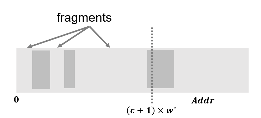 Figure 3: Memory layout at certain timestamp. Memory deallocation leaves fragments in memory space with lower address. Small requests tends to fit into these fragments with lower address.
2.2.1 Special case
To get the logarithmic, we first consider a special case where all requested memory size is exponent of 2. We shall prove that all such requested memory can be allocated at an address bounded by the logarithm of its size.
Let $l$ be the minimum integer satisfying $2^l\ge c \frac{W_{max}}{k}$, which means the jobs smaller then $2^l$ are so called ‘small jobs’ we talked above. We first prove a claim by induction.
Claim 2. A request of size $2^j, j\ge l$ can be allocated at an address not exceeding $(c+2+j-l)\times w^{\star}$.
Proof. We start with request of size $2^l$. We learn from Lemma 1 that after address $(c+1)\times w^{\star}$, the allocated size for each request is at least $2^l$. As a result, if there exists a fragment above that address, the fragments is at least $2^l$ since fragments are results of deallocated memory. By the definition of $w^{\star}$, there can not be a continuous memory space $>w^{\star}$ which is fully occupied. So the request of size $2^l$ can at least fit in a fragment before exceeding $(c+2)\times w^{\star}$.
For $j=l+1$, since the fragment above $(c+1)\times w^{\star}$ is at least $2^l$ and since there are $2w^{\star}$ between $(c+1)\times w^{\star}$ and $(c+3)\times w^{\star}$, we can find at least one fragment or continuous free space that $2^j$ can fit in, otherwise the portion of fragment and occupied space will lead to a contradiction with the definition of $w^{\star}$. Other induction steps are similar.
$\blacksquare$
We can derive from Claim 2 that the competitive ratio do not exceed $\frac{(c+2+j_{max}-l)\times w^{\star}}{w^{\star}}=c+2+j_{max}-l$, where $j_{max}=\log_2 W_{max}$ and $l = \lceil \log_2 (c \frac{W_{max}}{k})\rceil $.
\[Competitive \le c+2+\log_2 W_{max}-\lceil \log_2 (c \frac{W_{max}}{k})\rceil\le c+2- \log_2 c +\log_2 k\]Luby et al. [2] chose $c=4$, and derived a competitive ratio of $4+\log_2 k$.
2.2.2 General case
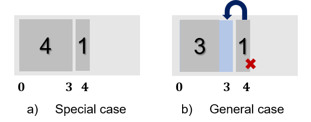 Figure 4: Demonstration of the reason why we can not use a scaling factor to directly derive general competitive ratio for First Fit from the special case. First Fit will put the request of size $1$ at address $3$, making a different decision from scaling the requests to the exponent of 2 to align with the special case.
For General cases, we first specify that we can not use an constant scaling factor to derive the competitive ratio from the special case. As shown in Figure 4, the First Fit algorithm will put a small request in the first available space, thus the decision results will be extremely different.
We give a technical lemma we will use about harmonic numbers $H_n=\sum_{i=1}^{n}\frac{1}{i}$.
Lemma 2. For $p\ge 1.5q$ and $q\ge 6$, $H_p-H_q\ge 0.3$.
Proof. A known bound of $H_n$ [7] is
\[H_n =\ln n+\gamma +\frac{1}{2n}-\frac{1}{12n^2}+\frac{1}{120n^4}-\epsilon\]$\gamma$ is Euler’s constant and $0<\epsilon<\frac{1}{256n^6}$. So
\[H_p-H_q\ge \ln \frac{p}{q} +\frac{1}{2p}-\frac{1}{2q} +\frac{1}{12q^2}-\frac{1}{12p^2}+\frac{1}{120p^4}-\frac{1}{120q^4}-\frac{1}{252p^6}\]Since $p\ge 1.5q$, $\frac{1}{12q^2}-\frac{1}{12p^2}\ge -(\frac{1}{120p^4}-\frac{1}{120q^4}-\frac{1}{252p^6})$.
So $H_p-H_q\ge \ln \frac{p}{q} +\frac{1}{2p}-\frac{1}{2q}> 0.3$ by $p\ge 1.5q$ and $q\ge 6$.
$\blacksquare$
The main idea is to find the upper bound for allocated memory address for requests of different size.
Claim 3. For request of size at most $j,\ j\ge \frac{W_{max}}{k} + 1$, the allocated address do not exceed
\[5w^{\star}+\frac{w^{\star}}{0.3}\sum_{i= \frac{W_{max}}{k} + 1}^{j}\frac{1}{i}\]Proof. We will prove by induction. By Lemma 1, we know that the claim holds for $j\le c\frac{W_{max}}{k}$. Assuming the claim holds for $j$, we will prove that it holds for $j+1$.
Let
\[L_i=(c+1)w^{\star}+\frac{w^{\star}}{0.3}\sum_{k= \frac{W_{max}}{k} + 1}^{i}\frac{1}{k}\]$L_i$ is the address upper bound of requests of size $i$ we want to prove. If for $j+1$, $L_{j+1}$ is not the upper bound, then by the definition of the algorithm, all fragments before $L_{j+1}$ are smaller than $j+1$.
We consider the portion of occupied space and fragments in the memory segmented by $L_i$. In the space between $L_i$ and $L_{i-1}$, where $\frac{W_{max}}{k} + 1\le i\le j+1$, the maximum fragment size is $j$ and the minimum occupied continuous space size is $i$. As a result the total occupied space between $L_i$ and $L_{i-1}$ is at least $\frac{i}{i+j}(L_i-L_{i-1})$.
Summing these up and we can get that the occupied space before $L_{j+1}$ is at least
\[\sum_{i=\frac{W_{max}}{k} + 1}^{j+1}\frac{i}{i+j}(L_i-L_{i-1})=\frac{w^{\star}}{0.3}\sum_{i=\frac{W_{max}}{k} + 1}^{j+1}\frac{1}{i+j}=\frac{w^{\star}}{0.3} \sum_{i=\frac{W_{max}}{k} +j+ 1}^{2j+1}\frac{1}{i}\]Chosing $c=4$, we have $j\ge 4\frac{W_{max}}{k}$ and thus $\frac{2j+1}{\frac{W_{max}}{k}+j+1}\ge 1.5$, with $\frac{W_{max}}{k}+j+1\ge 6$, we get from Lemma 2 that
\[\frac{w^{\star}}{0.3} \sum_{i=\frac{W_{max}}{k} +j+ 1}^{2j+1}\frac{1}{i}\ge w^{\star}\]which contradicts the definition of $w^{\star}$. So $L_{j+1}$ is the upper bound as we chose $c=4$.
$\blacksquare$
By Claim 3, we have the maximum memory space $M$ for First Fit satisfies
\[M\le 5w^{\star}+\frac{w^{\star}}{0.3}\sum_{i=\frac{W_{max}}{k} + 1}^{W_{max}}\frac{1}{i}\le 5w^{\star}+\frac{w^{\star}}{0.3}\left(1+\ln\left(\frac{W_{max}}{1+\frac{W_{max}}{k} }\right)\right)\le w^{\star}(9+4\ln k)\]So the competitive ratio is $9+4\ln k$.
3. The Coloring Algorithm
Now, we introduce one of segregated storage methods for DMA. This algorithm [2] is called The Coloring algorithm.
3.1 Algorithm Overview
The algorithm classify the requests according to their size. Specifically, Each request of size $l$ will be classified as $\lceil \log_2 (l) \rceil$ type.
For type $t$, several memory segments of size $2^t$ are assigned to it. Every time we receive a request of $t_i$ type, we try to find a free segment assigned to $t_i$ and allocate requested space in that segment. If no such free segments exists, we will assign a new segment of size $2^{t_i}$ to type $t_i$ and allocate space for the request in that new segment. Once we assign a segment to certain type, it will be reserved after the requested space is deallocated.
3.2 Competitive Analysis
Some notes for this analysis
- Classifying requests of different size into different types and allocate memory for each kind simplify the analysis.
- Refined results can be obtained through the sub-case discussion
To analysis the competitive ratio for The Coloring algorithm, we define the maximum concurrent request number for each type $t_i$ as $k_{t_i}$.
For each request classified as different type and allocated in a segment belonging to that type, we know that the memory space exclusive to that request is at most twice as needed. For each type, the number of segments assigned to is is $k_{t_i}$, so the total memory assigned to it is $k_{t_i}\times 2^{t_i}\le 2w^{\star}$.
Since we classify by request size and the maximum size is $W_{max}$, there are at most $\lceil \log_2 (W_{max}) \rceil$ types. So $ALG\le \lceil \log_2 (W_{max}) \rceil \times 2 \times w^{\star}$. So the competitive ratio is $O(\log(W_{max}))$.
Another analysis yields a competitive ratio for The Coloring algorithm of $O(\log k)$.
The types can be further divided into two categories,
-
Type $t_i$ satisfying $2^{t_i}\le \frac{W_{max}}{k}$.
The total memory space needed by this kind is $\sum_{t=0,2^{t}\le \frac{W_{max}}{k} } 2^t k_t\le \sum_{t=0,2^{t}\le \frac{W_{max}}{k} } 2^t k\le 2k\frac{W_{max}}{k}=2W_{max}$.
-
Type $t_i$ satisfying $2^{t_i}\ge \frac{W_{max}}{k}$.
The total memory space needed by this kind is at most $2w^{\star}\times num$, $num$ is the number of types of this kind. Since $2^{t_i}\ge \frac{W_{max}}{k}$, $num$ is $O(\log(k))$. With fixed constant $c$ such that $num \le c \cdot \log(k)$, $2w^{\star}\times num\le c \cdot \log(k)\cdot 2w^{\star}$.
So $ALG\le 2W_{max}+c \cdot \log(k)\cdot 2w^{\star}$. The competitive ratio is $\frac{ALG}{OPT}=2c\cdot \log(k)+\frac{2W_{max}}{w^{\star}}$, can be bounded by $O(\log k)$.
Putting all above analysis together, the competitive ratio is $\min\lbrace\Theta (\log W_{max}),\Theta (\log k)\rbrace$.
3.3 Comparison
Luby et al. [2] compared Coloring Algorithm with First Fit and indicated that the performance of these two algorithms depends on the application. They found that for each algorithm, there exist cases that one is near optimal while the other each the worst case bound. However, besides that the two algorithms perform comparably when it comes to minimizing memory waste, it is worth noting that Coloring Algorithm is generally more efficient than First Fit when it comes to searching for allocation space.
4. The Buddy System
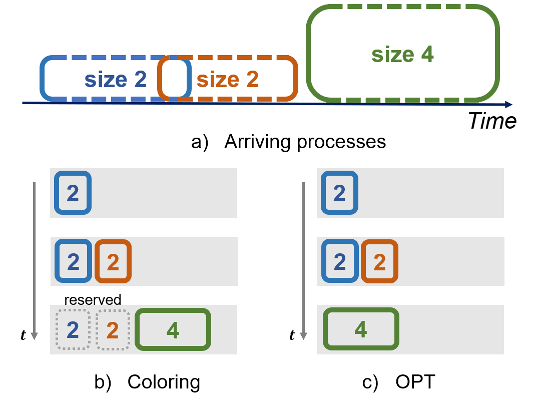 Figure 5: An example that the Coloring Algorithm waste space because it reserve assigned segments for each type.
Coloring Algorithm is a efficient online DSA algorithm, however, we can see that reserving the assigned segments for each type can be wasting. Figure 5 gives an simple example. $OPT$ can reuse the space in $[0,3]$ for the third request and use memory of size $4$ to serve the $3$ requests. Coloring Algorithm first assigned $[0,1]$ and $[2,3]$ to the first and second request, after these memory are deallocated, Coloring Algorithm reserve them for type $t=1$. When the third request arrive, it will assigned $[4,7]$ to type $t=2$ and use memory of size $8$ to serve the $3$ requests.
The Buddy System is more flexible and able to conduct some reuse.
4.1 Algorithm Overview
The Buddy System will divide original memory into halves recursively according certain rules about divided sizes. When a request arrive, it will round up the size to the minimum divided size $s_d$ that can handle the request. Then, it tries to find a free segment of size $s_d$. If if find one, the segment will be used to serve that request. Otherwise, it will divide a larger segment recursively to get a segment of size $s_d$. When a memory space is deallocated, the corresponding segments will be freed. The Buddy System will check its ‘buddy’ (the other segment divided from the same parent). If the ‘buddy’ is also free, these two segment will merge back to their parent segment. The merging precess follows a bottom-up approach and stop until the ‘buddy’ is not free or it reaches the root. An example of Buddy System allocating a memory of size $16$ for the requests in Figure 5 can be found in Figure 6.
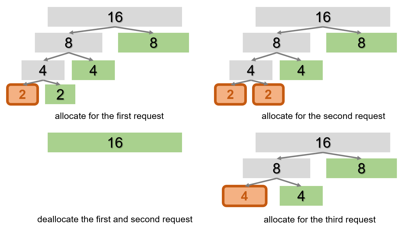 Figure 6: A simple example of Binary Buddy System. The green segments are free and the orange segments are occupied to serve the requests. Note that in this example, Binary Buddy System overcome the waste shown in Coloring Algorithm.
The original Buddy System divide the segments into sub-segments whose sizes are powers of 2. This kind of Buddy System is called Binary Buddy System [9]. Figure 6 is an example of Binary Buddy System. Other variations includes Fibonacci Buddy System [8], using Fibonacci number as segments’ size.
Robson [6] indicated that with Buddy System, a memory of size $2w^{\star}\log_2(W_{max})$ is enough to serve the requests with distribution we discussed in these notes. The Buddy System is a widely used DMA algorithm, the Linux kernel also employs the buddy system with modifications.
5. Experiment
We implement a simple simulator in Python to evaluate memory allocation performance across various dynamic memory allocation (DMA) algorithms. The algorithms considered in this study include the following:
- First Fit in Section 2.
- Best Fit, another traditional heuristics that searches for the block that best matches the process’s requirements, aiming to leave the smallest possible fragment of unused memory.
- Coloring Algorithm in Section 3.
- Binary Buddy System in Section 4.
To ensure a meaningful comparison, we divide these algorithms into two categories and analyze each category separately. Traditional heuristics like First Fit and Best Fit rely on brute force search to allocate memory, resulting in significant searching overhead. In contrast, the Coloring Algorithm and Binary Buddy System optimize search efficiency but introduce additional overhead related to memory utilization. Consequently, direct comparison across all algorithms is inappropriate due to these fundamental differences.
We evaluate the algorithms under varying numbers of requests and diverse request size distributions. The request sequence is generated by a pseudo-random number generator with fixed random seed. The size of requests is a uniform distribution from $1$ to $m$ or a exponential distribution with mean $\frac{m}{2}$ truncated to $[1,m]$. A uniformly distributed lifetime is assigned to each request.
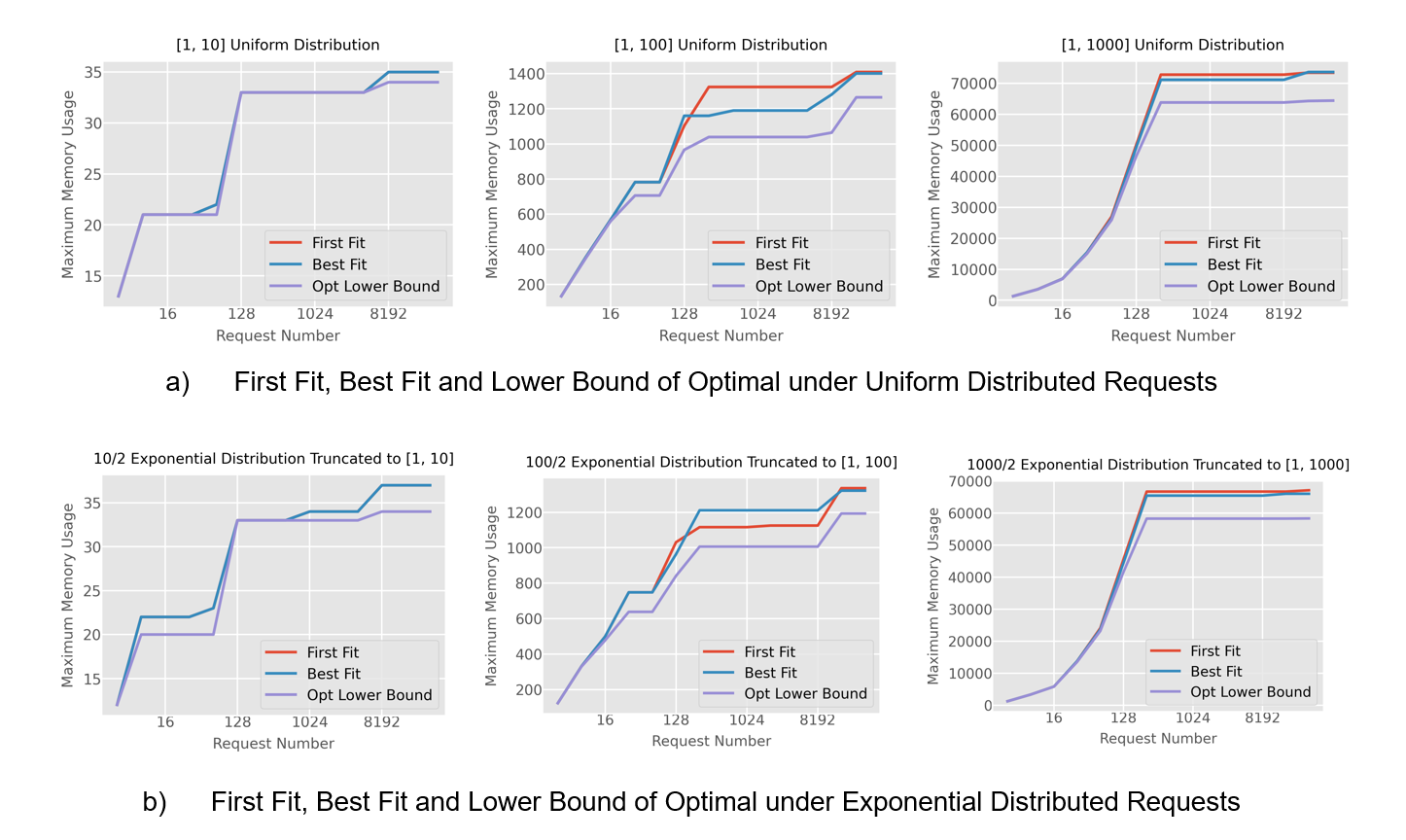 Figure 7: Maximum memory usage of FirstFit, BestFit and lower bound of optimal under different distributed requests.
Figure 7 gives the result of maximum memory usage of traditional heuristics. We can learn from the curve that under both uniform distribution and exponential distribution, the maximum memory usage of both algorithms are close to the optimal lower bound, with a overhead not exceeding $23\%$. Also, we find that the maximum memory usage of the two algorithms exhibit no significant superiority or inferiority. Their performance is comparable and each demonstrates distinct advantages under different scenarios. However, we observe significant overhead in searching for memory space to fulfill requests, particularly as $m$ increases in both distributions. This excessive overhead renders these algorithms unsuitable for complex, real-world serving scenarios.
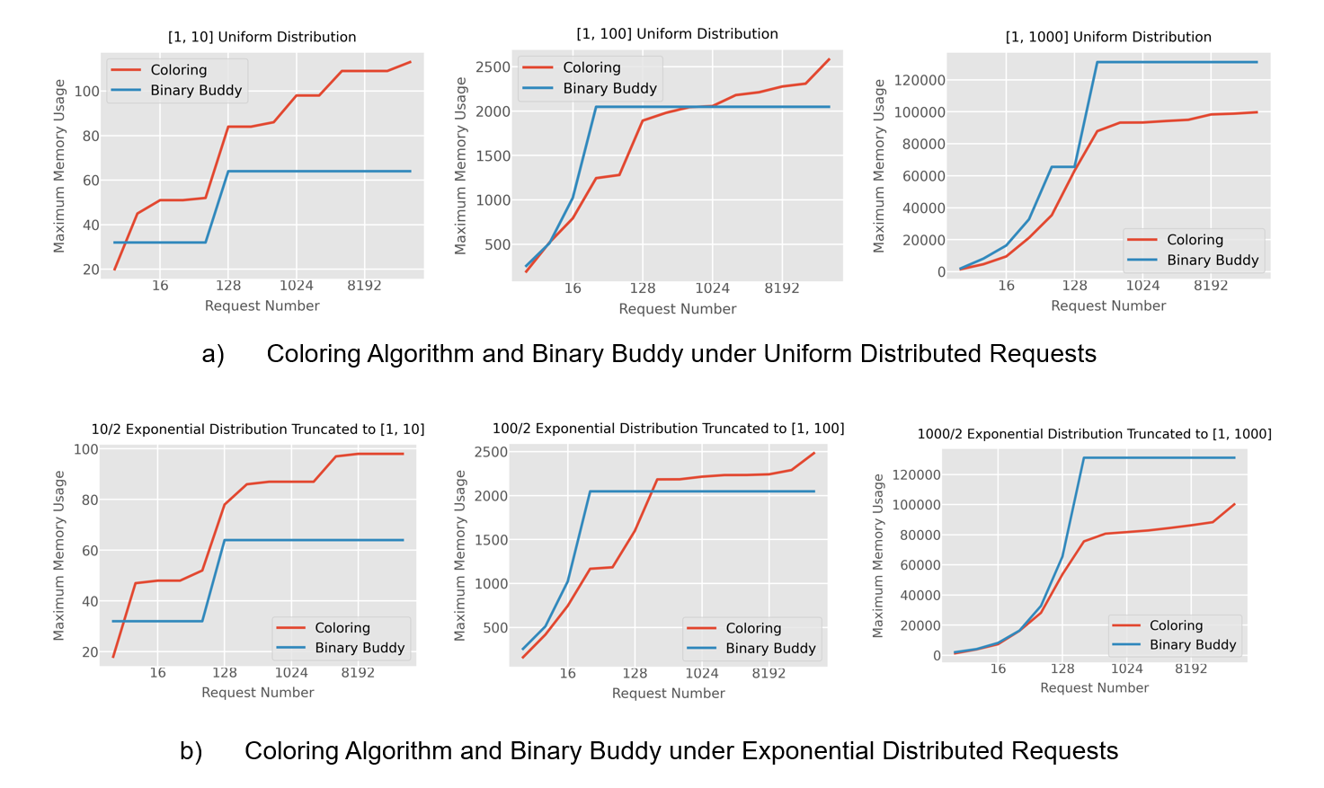 Figure 8: Maximum memory usage of The Coloring Algorithm and Binary Buddy System under different distributed requests.
For the Coloring Algorithm and the Binary Buddy System, Figure 8 shows that under both distributions, the maximum memory usage of the Binary Buddy System converges quickly as the number of requests increases. In contrast, the maximum memory usage of the Coloring Algorithm continues to grow. As $m$ increases, we observe that the Binary Buddy System generally performs worse. This decline is primarily due to our straightforward implementation, where the maximum memory is doubled when sufficient space cannot be found. This doubling often results in significant external fragmentation.
The distributions we selected are truncated to a narrow range, which significantly impacts the behavior of the allocation algorithms. Under such constraints, the Binary Buddy System exhibits a substantial increase in memory usage when the current memory utilization is high as a result of its doubling mechanism, which allocates additional memory in powers of two. In contrast, the Coloring Algorithm demonstrates a more efficient approach to memory expansion under our constraints. It increases memory usage only by the smallest power of two that is no less than the largest request size. This adaptive scaling minimizes unnecessary memory allocation.
6. Conclusion
In these notes, we surveyed some commonly used online algorithms for Dynamic Memory Allocation (DMA) problem. We analyzed their competitive ratio, traditional heuristics like First Fit has a competitive ratio of $\min\lbrace\Theta (\log W_{max}),\Theta (\log k)\rbrace$. And segregated storage methods like Coloring Algorithm also has a competitive ratio of $\min\lbrace\Theta (\log W_{max}),\Theta (\log k)\rbrace$.
We implemented four of these algorithms and do simulation experiment to evaluate the efficiency of them.
References
[1] Weinstock, Charles B., and William A. Wulf. “An efficient algorithm for heap storage allocation.” ACM Sigplan Notices 23.10 (1988): 141-148.
[2] Luby, Michael G., Joseph Naor, and Ariel Orda. “Tight bounds for dynamic storage allocation.” SIAM Journal on Discrete Mathematics 9.1 (1996): 155-166.
[3] Naor, Joseph Seffi, Ariel Orda, and Yael Petruschka. “Dynamic storage allocation with known durations.” Discrete Applied Mathematics 100.3 (2000): 203-213.
[4] Puaut, Isabelle. “Real-time performance of dynamic memory allocation algorithms.” Proceedings 14th Euromicro Conference on Real-Time Systems. Euromicro RTS 2002. IEEE, 2002.
[5] Hartmanis, Juris. “Computers and intractability: a guide to the theory of np-completeness (michael r. garey and david s. johnson).” Siam Review 24.1 (1982): 90.
[6] Robson, John M. “Worst case fragmentation of first fit and best fit storage allocation strategies.” The Computer Journal 20.3 (1977): 242-244.
[7] Knuth, Donald E. The Art of Computer Programming: Fundamental Algorithms, Volume 1. Addison-Wesley Professional, 1997.
[8] Hirschberg, Daniel S. “A class of dynamic memory allocation algorithms.” Communications of the ACM 16.10 (1973): 615-618.
[9] Knowlton, Kenneth C. “A fast storage allocator.” Communications of the ACM 8.10 (1965): 623-624.