We consider the $Makespan$ problem for identical machines. There are $m$ identical machines and a sequence of $n$ jobs arriving in order to be processed. Each job is of size $p_i$, which indicates the time needed to process the job on single machine. Every job can only be processed once on one machine. We need an algorithm to assign a job to a machine immediately after the job arrives, without any knowledge of future jobs. The $makespan$ of one machine is the sum of the size of jobs processed on it. And the $Makespan$ is the maximum of all $m$ machines’ $makespan$, we want to minimize $Makespan$.
Formally, this can be defined as
Makespan Minimization
Input: the number of identical machines $m$, the number of jobs $n$, $(p_1,\ p_2,\ \dots,\ p_n)$ where $p_i > 0$ is the processing time of job $j_i$.
Output: an assignment $\mathcal{A}:\lbrace 1,2,\dots,n\rbrace \to\lbrace 1,2,\dots,m\rbrace$ form the $n$ jobs to the $m$ machines.
Objective: find an assignment $\mathcal{A}$ to minimize $Makespan=\max{\sum_{j:\mathcal{A}(i)=j}p_i}$.
1. List Arrival
We first consider a simple model. Assume that the job list is known at time $0$, we can not schedule these jobs out of order, but we can schedule the next job as soon as we have an idle machine. We define this model as $List\ Arrivel$ Identical Machine Makespan Minimization.
List Arrival Makespan Minimization
Input: the number of identical machines $m$, the number of jobs $n$, the job list $(j_1,\ j_2,\ \dots,\ j_n)$ indicating jobs arriving one by one, $(p_1,\ p_2,\ \dots,\ p_n)$ where $p_i > 0$ is the processing time of job $j_i$.
Output: an assignment $\mathcal{A}:\lbrace 1,2,\dots,n\rbrace\to\lbrace 1,2,\dots,m\rbrace$ form the $n$ jobs to the $m$ machines.
Objective: find an assignment $\mathcal{A}$ to minimize $Makespan=\max{\sum_{j:\mathcal{A}(i)=j}p_i}$.
1.1 Greedy Algorithm
Greedy algorithm is what first come to our mind.
Assign the arriving job onto the machine with earliest finishing time at that timestamp.
1.1.1 Competitive Analysis
Theorem 1. For all $m$ and all input sequences $(p_1,\ p_2,\ \dots,\ p_n)$, the competitive ratio is $2-\frac{1}{m}$.
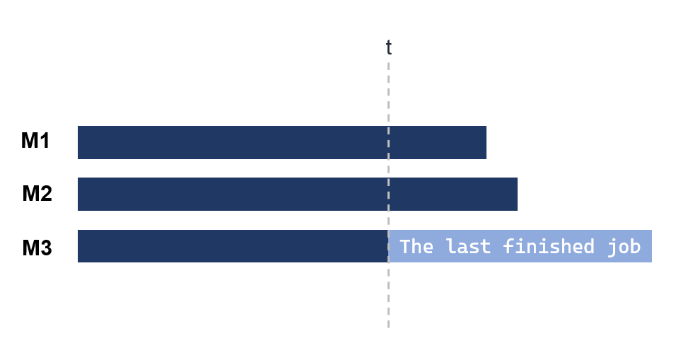 Figure 1: Proof Demonstration
Proof. As demonstrate in Figure 1. Consider the last finished job $j_n$, and it needs $p_n$ to be processed. We can assume that this job is the last scheduled job since if there are other jobs arriving after $j_n$, $ALG$ remains unchanged and $OPT$ may become worse. $j_n$ starts being processed at $t$, so $ALG=t+p_n$ The total working time of the jobs arrive before $j_n$ is at least $mt$ since $j_n$ was assign to be processed on the earliest finished machine at that time. As a result, $OPT\ge \frac{mt+p_n}{m}=t+\frac{p_n}{m}$. Also, since $j_n$ needs to be processed on one machine, $OPT\ge p_n$ So $ALG-OPT\le (1-\frac{1}{m})p_n\le (1-\frac{1}{m})OPT$.
\[\frac{ALG}{OPT}=1+\frac{ALG-OPT}{OPT}\le2-\frac{1}{m}\]$\blacksquare$
Note that this analysis is tight, a counter example is a sequence of $m(m-1)$ jobs of size $1$ followed by one job of size $m$.
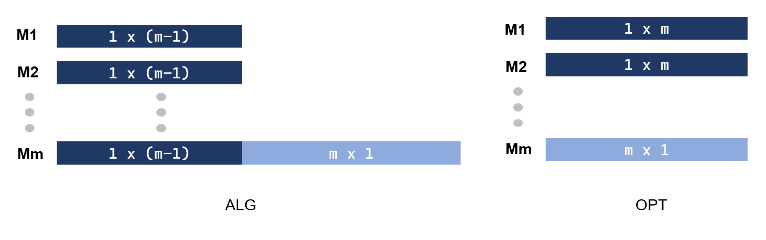 Figure 2: Counter Example of Greedy Algorithm
As shown in Figure 2, $ALG$ will assign the $m(m-1)$ jobs equally on the $m$ machines and assign the last one to arbitrary one, so $ALG=2m-1$. $OPT$ will assign the $m(m-1)$ jobs on $m-1$ machines and the last job on one machine, so $OPT=m$. $\frac{ALG}{OPT}=\frac{2m-1}{m}=2-\frac{1}{m}$.
Also note that when $m=2$, greedy is the the best deterministic algorithm. If at first come 2 jobs of size $1$, assign them to the first machine break the ratio since $ALG=2$ while $OPT=1$. If we assign them to different machines, then, if the third arriving job is of size $2$, then $ALG=3$ while $OPT=2$, so the ratio is $1.5=2-\frac{1}{m}$.
1.2 MR Algorithm
We proved that greedy has competitive ratio $2-\frac{1}{m}$ and this is the best deterministic algorithm when $m=2$. Now, the question is how to beat $2$ when $m\to \infty$. Taking a closer look at the counter example of greedy algorithm in Figure 2, we can find that if all the machines have the same load when a heavy job arrive, there will be a terrible cost. Greedy tends to make the machines flat, but making them a little steeper may be beneficial.
MR Algorithm [1] is based on this idea of making flat schedules steeper by scheduling jobs on some medium-loaded machine.
1.2.1 Notation
We first define some notation and parameters we will use in this algorithm. Assume that we sort all the machines in decreasing order of current finishing time every time we need to schedule an arriving job. The sorted machines at time $t$ are labeled $\lbrace M_1^t,\ M_2^t,\cdots,\ M_m^t\rbrace$ and finishing time of $M_i^t$ is $l_i^t$. For $j=1,\ 2, \cdots,\ m$, let $D_j^t$ be the average finishing time of $M_j^t,\cdots,\ M_m^t$, so $D_j^t=\frac{1}{m-j+1}\cdot\sum_{k=j}^{m}l_k^t$. To achieve the competitive ratio $c$, we define $i=\left\lceil \frac{5c-2c^2-1}{c}\cdot m\right\rceil -1$ and $k=2i-m$. In the paper [1], the author shows that MR works well if we choose $c\ge 1+\sqrt{\frac{1+\ln 2}{2}}$ and explains the magic number $i$.
We call MR’s schedule $flat$ at $t$ if $l_k^{t-1}<\frac{2(c-1)}{2c-3} \cdot D_{i+1}^{t-1}$, otherwise, we call MR’s schedule $steep$. If at time $t$, the arriving job $j_q$ is so heavy that $p_q+l_i^{t-1}>c\cdot D_1^t$, we call MR’s schedule $dangerous$, indicating that this may break our targeting competitive ratio.
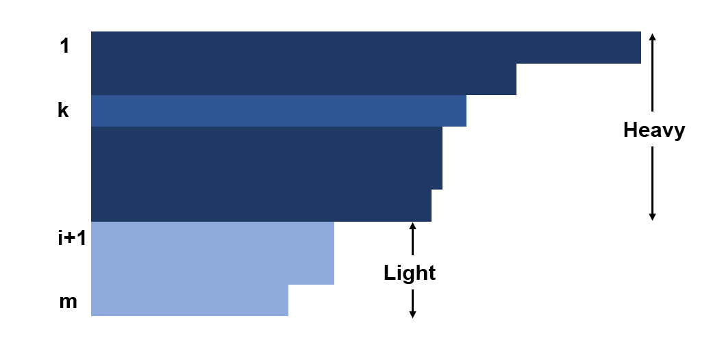 Figure 3: MR Algorithm Sample
Figure 3 gives a sample of the sorted machines at time $t$, the parameters $k,\ i$ are used in labeling. Intuitively, we can view the machines $M_1^t,\ M_2^t,\cdots,\ M_i^t$ as having $Heavy$ workload, and the remaining ones having $Light$ workload. And $M_k^t$ is used to indicate whether the machines are $steep$.
1.2.2 Algorithm
The algorithm schedule the arriving job on either $M_m^{t-1}$ or $M_i^{t-1}$ based on the flatness.
Let $p_q$ be the processing time of the arriving job $j_q$, if the current schedule is $steep$ or $dangerous$,
we assign $j_q$ to the lightest machine $M_m^{t-1}$.
Otherwise, we assign it to $M_i^{t-1}$
1.2.3 Analysis Sketch
The main idea is to prove that there are many large jobs so that $OPT$ have to process more than one large jobs on the same machine, and this gives $ALG$ a chance to catch up.
Consider the job that will break the targeting competitive ratio $c$, we call it the last job $j_n$. Assume that the last job is scheduled at $t$, this job will be assigned to the last or the lightest machine by algorithm definition.
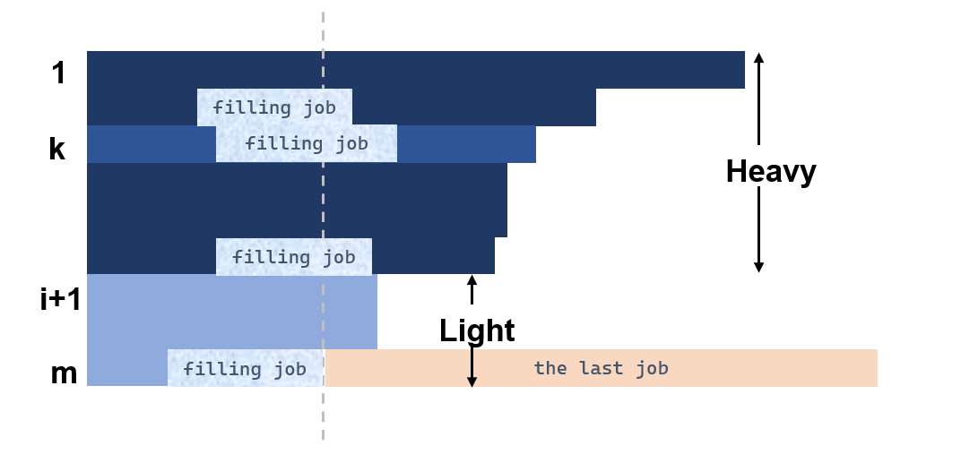 Figure 4: MR Algorithm Proof Illustration
Figure 4 gives an illustration of the last job.
Lemma 1. The last job $j_n$ is scheduled when MR’s schedule is $flat$.
Proof. We prove by contradiction.
If the schedule is $steep$, then $l_k^{t-1}\ge \frac{2(c-1)}{2c-3} \cdot D_{i+1}^{t-1}$. Since $l_m^{t-1}\le D_{i+1}^{t-1}\le \frac{2c-3}{2(c-1)} \cdot l_k^{t-1}$ and the total workload is at least $l_m^{t-1}\cdot (m-k)+l_k^{t-1}\cdot k$, we have
\[OPT \ge \frac{l_m^{t-1}\cdot (m-k)+l_k^{t-1}\cdot k}{m} \ge \frac{m-k+k\frac{2(c-1)}{2c-3}}{m} \cdot l_m^{t-1}=(1+\frac{k}{(2c-3)m})\cdot l_m^{t-1}\]Also, since $j_n$ needs to be processed on one machine,
\[OPT\ge p_n\]Since $j_n$ is the job that break the competitive ratio, we have
\[l_m^{t-1}+p_n > c\cdot OPT\]Let $c=1+\sqrt{\frac{1+\ln 2}{2}}\approx 1.9201$, then $k\approx 0.278m$. So
\[OPT\ge (1+\frac{k}{(2c-3)m})\cdot l_m^{t-1} = (1+\frac{0.278}{2*1.9201-3})\cdot l_m^{t-1}\ge (1.33\times 0.9201)\cdot OPT>OPT\]is a contradiction.
$\blacksquare$
We proved that the schedule is $flat$ at $t$ before the last job $j_n$ was assigned, and the lightest machine has workload $l_m^{t-1}$.
We call the jobs making the workload increase to $l_m^{t-1}$ as the $filling\ job$ on that machine. Some examples of $filling\ job$s can be found in Figure 4.
For $q = 0,\ 1, \cdots,\ m$, let $t_q$ be the time the $q$-th $filling\ job$ arrive. Its clear that at that time, $M_q^{t_q},\ M_{q+1}^{t_q},\cdots,\ M_m^{t_q}$ are the ones having workload less than $l_m^{t-1}$. We define the average load of these machines at $t_q$ as $D_{q}$. Since after receiving $i$ $filling\ job$s, the following $filling\ job$s can only be assigned to the lightest machines at that time, $D_{i+1}\le\cdots\le D_m$.
We give the following claim.
Claim 1. For all $q>i$, $D_{q} < l_m^{t-1} - \frac{l_m^{t-1}}{2(c-1)}$.
The proof of this claim can be found in the paper [1].
We define the jobs which needs at least $\frac{l_m^{t-1}}{2(c-1)}$ to process as $heavy$. Note that above claim somehow implies that the $filling\ job$s of the light machine are $heavy$.
Lemma 2. There are at least $m+1$ $heavy$ jobs $\lbrace j_{t^1},\ j_{t^2}, \cdots,j_{t^{m+1}}\rbrace$ such that $p_{t^i}\ge \frac{l_m^{t-1}}{2(c-1)}$.
Proof. First, since $l_m^{t-1}+p_n > c\cdot OPT$ and $OPT> l_m^{t-1}$, $p_n >(c-1)l_m^{t-1}>\frac{l_m^{t-1}}{2(c-1)}$, so $j_n$ is $heavy$.
Then, we look back from $t$. We proved that $j_n$ is scheduled when the schedule is $flat$, So we can find some of the last $filling\ job$s, possibly 0, are also scheduled when the schedule is $flat$. Assume these $filling\ job$s are ${j_{t_{s+1}},\ j_{t_{s+2}},\cdots,\ j_{t_m}}$ where $s\ge i$. These jobs are assign on the lightest machine since another option is already full. By the algorithm, when the schedule is $flat$, we only assign the job to the lightest machine because it is $dangerous$. That is $p_{t_q}+l_i^{t-1}>c\cdot D_1^{t_q}$. After assigning the $filling\ job$, we have $i$ machines with workload at least $l_i^{t_q-1}$, one at least $l_m^{t-1}$, and $(m-i-1)$ at least $(l_m^{t-1}-\frac{l_m^{t-1}}{2(c-1)})$ since they are heavier than the lightest machine. So
\[D_1^{t_q}\ge \frac{i\cdot l_i^{t_q-1}+l_m^{t-1}+(m-i-1)(l_m^{t-1}-\frac{l_m^{t-1}}{2(c-1)})}{m}\]As a result, we can get $p_{t_q}>\frac{l_m^{t-1}}{2(c-1)}$ after some calculation, and this means that $\lbrace j_{t_{s+1}},\ j_{t_{s+2}},\cdots,\ j_{t_m}\rbrace$ are $heavy$.
For the rest of the $filling\ job$s, $\lbrace j_{t_{i+1}},\ j_{t_{i+2}},\cdots,\ j_{t_s}\rbrace$ are assigned to the lightest for the same reason as above, by our claim, we have $\forall q>i, D_{q} < l_m^{t-1} - \frac{l_m^{t-1}}{2(c-1)}$, so we have the same result as above situation and $\lbrace j_{t_{i+1}},\ j_{t_{i+2}},\cdots,\ j_{t_s}\rbrace$ are $heavy$. For $\lbrace j_{t_{k+1}},\ j_{t_{k+2}},\cdots,\ j_{i}\rbrace$, since no job will be assign to $M_k^{t_q}$ after $t_k$, we know that
\[l_k^{t_q-1}\ge l_m^{t-1}=\frac{2(c-1)}{2c-3}\cdot (l_m^{t-1} - \frac{l_m^{t-1}}{2(c-1)})\]By the chain, we have $l_m^{t-1} - \frac{l_m^{t-1}}{2(c-1)}>D_{i+1}>D_{i+1}^{t_q-1}$. So
\[l_k^{t_q-1}\ge\frac{2(c-1)}{2c-3}\cdot D_{i+1}^{t_q-1}\]These means that the schedule before assign the job is $steep$, so the $filling\ job$ will be assigned on the lightest machine. We can thus prove these jobs are $heavy$ in a similar way.
At last, we consider $\lbrace j_{t_1},\ j_{t_2},\cdots,\ j_{k}\rbrace$. For the $q$-th job arriving at $t_q$, we have
\[l_m^{t_q-1}\le l_i^{t_q-1}\le l_i^k\le l_m^{t_i}\le D_{i+1}<l_m^{t-1} - \frac{l_m^{t-1}}{2(c-1)}\]So these jobs are $heavy$.
In conclusion, all the $filling\ job$s are $heavy$.
Since there are $m$ $filling\ job$s, we have $m$ $heavy$ jobs besides $j_n$, so we have at least $m+1$ $heavy$ jobs in total.
$\blacksquare$
The $m+1$ $heavy$ jobs need to be assigned to $m$ identical machines, so at least one machine needs to process 2 $heavy$ jobs. So $OPT\ge 2\cdot\frac{l_m^{t-1}}{2(c-1)}=\frac{l_m^{t-1}}{c-1}$ and $ALG=l_m^{t-1}+p_n\le (c-1)OPT+OPT=c\cdot OPT$. So the competitive ratio is $c$ since
\[\frac{ALG}{OPT}\le \frac{c\cdot OPT}{OPT}=c\]MR works well if we choose $c\ge 1+\sqrt{\frac{1+\ln 2}{2}}\approx 1.9201$, so it can beat the $2$-competitive greedy algorithm.
2. Real-time Arrival
Now, we consider a more complex model. The jobs arrive at a specific time, and we can only schedule the job after the arriving time.
Makespan Minimization
Input: the number of identical machines $m$, the number of jobs $n$, the $i$-th job $j_i$ arrive at $r_i$ and need $p_i$ to process.
Output: an assignment $\mathcal{A}:\lbrace 1,2,\dots,n\rbrace\to\lbrace 1,2,\dots,m\rbrace$ form the $n$ jobs to the $m$ machines.
Objective: find an assignment $\mathcal{A}$ to minimize $Makespan=\max{\sum_{j:\mathcal{A}(i)=j}p_i}$.
Note that in this model $OPT$ knows that $j_i$ will arrive at $t_i$, but it can not schedule the job to be processed before $t_i$.
2.1 Greedy Algorithm
We can try greedy again on this model.
Similar to our greedy algorithm used in the $List\ Arrival$, we can simply assign the arriving job to the current least busy machine. With a similar analysis approach, we can see that greedy is $2$-competitive.
2.2 LPT Algorithm
But, since this job may be stalled for a while, we can make a little optimization. If other heavier jobs arrive during that time period, we can withdraw that job and schedule the heaviest one onto the least busy machine.
This intuition comes from the off-line optimal algorithm for $Makespan\ Minimization$. An example may reveal the strength of this optimization. Look back at our counter example for the greedy algorithm in $List\ Arrival$ in Figure 2, If the job $j_i$ with size $m$ arrive at $0$, it will be scheduled immediately. If it arrive at $t_i>0$, it will be scheduled after some jobs of size $1$, but $OPT$ will have a larger overhead as well.
More specifically, the optimized greedy algorithm is as follows.
When a machine $M_i$ is free at $t$, we schedule the heaviest pending job to $M_i$ at $t$.
2.2.1 Competitive Analysis
We will prove that the competitive ratio of algorithm is $1.5$.
Consider the last finished job $j_n$, without lose of generality, it is the last scheduled job.
We first consider the case that the machines are always full before $j_n$ was scheduled.
Since all the machines are full before $t_n$, the total workload is at least $m\cdot t_n$. So
\[OPT \ge t_n\]If $p_n\le 0.5OPT$, then $ALG=t_n+p_n\le1.5OPT$.
If $p_n>0.5OPT$, we prove that $ALG\le 1.5OPT$ by contradiction.
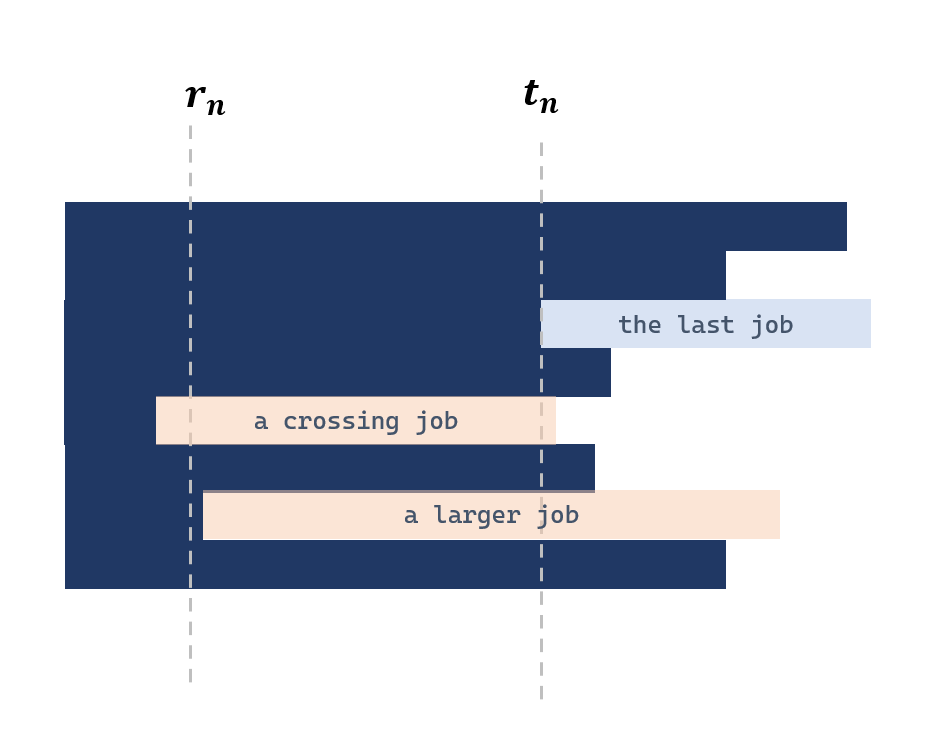 Figure 5: LPT Algorithm Proof Illustration
Assume $ALG > 1.5OPT$, consider the time period between $r_n$, $j_n$’s arriving time, and $t_n$, $j_n$’s schedule time, $j_n$ is not scheduled to any machine for $2$ possible reasons as shown in Figure 5.
- There is a crossing job. This means that there is a job processes on the machine between $r_n$ and $t_n$. In this case, if the ratio is broken, we need $ALG=t_n+p_n>1.5OPT$. Since $OPT\ge p_n+r_n$, we get $t_n-r_n\ge 0.5OPT$. The crossing job $j_i$ satisfies that $p_i>t_n-r_n\ge 0.5OPT$.
- There is a larger job that need to be scheduled before $j_n$. In this case $p_i\ge p_n> 0.5 OPT$.
So there are at least $m+1$ jobs larger than $0.5OPT$ and at least $2$ such job will be scheduled to one machine. So we have $OPT> 2\times 0.5 OPT=OPT$ which is a contradiction.
Now, we consider some machines may be idle before $j_n$ was scheduled. Assume $t’$ is the last idle time as shown in Figure 6, so all the machines are full between $t’$ and $t_n$.
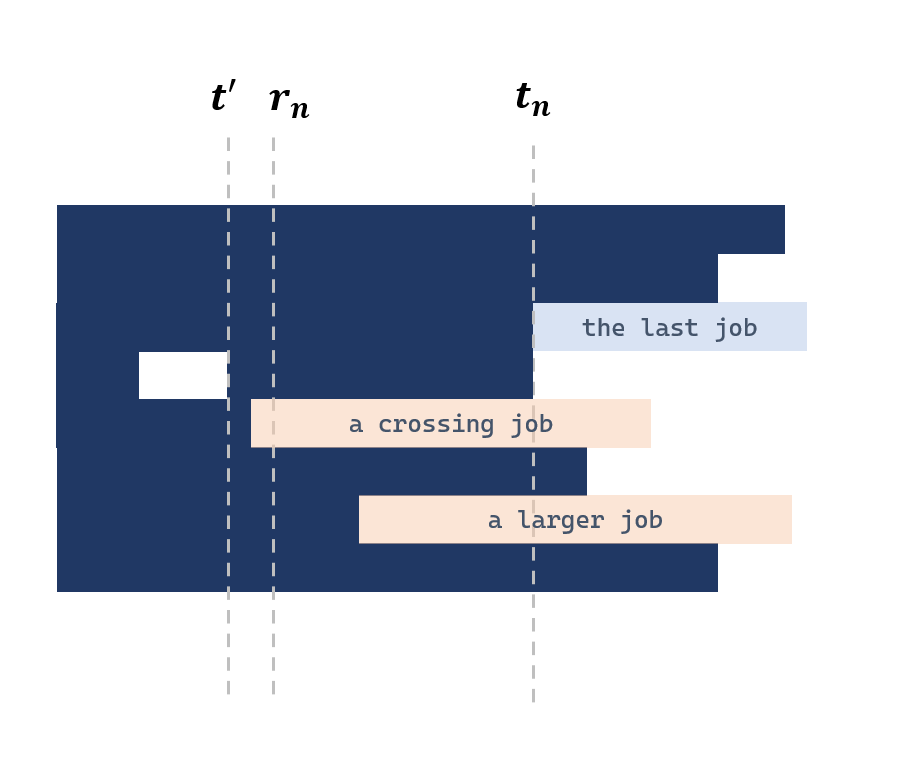 Figure 6: LPT Algorithm with Idle Time
It’s clear that $r_n\ge t’$, since the algorithm will schedule a job if there is an idle machine.
We still have $m$ large jobs either larger than $j_n$ or cross $r_n$ and $t_n$. More specifically, there jobs are
- A crossing job. This means that there is a job processes on the machine between $r_n$ and $t_n$. In this case, if the ratio is broken, we need $ALG=t_n+p_n>1.5OPT$. Since $OPT\ge p_n+r_n$, we still get $t_n-r_n\ge 0.5OPT$. The crossing job $j_i$ satisfies that $p_i>t_n-r_n\ge 0.5OPT$.
- A larger job that need to be scheduled before $j_n$. In this case $p_i\ge p_n> 0.5 OPT$.
We first prove that $OPT$ schedules all the $m$ large jobs after $t’$ by contradiction.
If $OPT$ schedules some of these jobs before $t’$, $OPT$ will put at least $2$ of these jobs one the same machine. Assume the jobs are $j_a$ and $j_b$ as illustrated in Figure 7.
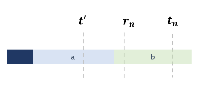 Figure 7: OPT Schedule Before t’
We have
\[r_a+p_a+p_b\le OPT\]Assume $ALG$ schedules $j_a$ at $t_a$. By our define of the large $m+1$ jobs, we have $t_a+p_a\ge t$. So
\[ALG= t_n +p_n \le t_a+p_a +p_n\]If $ALG\ge 1.5 OPT$, then
\[t_a+p_a +p_n \ge 1.5 OPT\]Since $p_b> p_n$, we can get
\[t_a-r_a\le 0.5OPT\]Which means the job $j_a$ will have a delay of at least $0.5OPT$ in $ALG$.
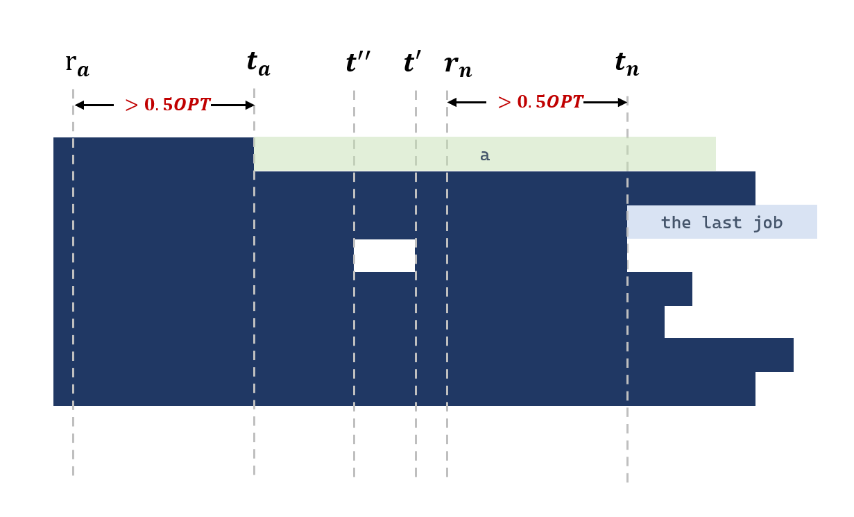 Figure 8: ALG’s View
Putting all these things together in $ALG$, we have a delay of at least $0.5OPT$ before $t’$ and a delay of at least $0.5OPT$ after $t’$. Since all the machines are full during each delay by the algorithm, we know the total workload is $> m\cdot (0.5OPT+0.5OPT)$. So $OPT>\frac{m\cdot(0.5OPT+0.5OPT)}{m}=OPT$, which is a contradiction. So $OPT$ schedules all the $m$ large jobs after $t’$.
If $OPT$ schedules these $m$ jobs after $t’$, $OPT\ge t’+ \frac{m(t_n-t’)}{m}=t_n$ and $ALG=t_n+p_n$. $p_n$’s bound can be refined to $p_n\le \frac{1}{2}(OPT-t’)$ since previous bound is from our assumption that the last idle time is $0$ and now we refine that to $t’$. If $OPT$ schedule all the jobs $ALG$ schedule after $t’$ after $t’$ as well, the $1.5$ ratio holds in a similar manner. So we need to consider that some $OPT$ may schedule some of these jobs before $t’$ and gain a smaller $Makespan$. These jobs must arrive before $t’’$. We pick the job $j_d$ that is delayed the most. Since $OPT$ schedules it earlier, assume it delayed $\delta$ less. So $OPT$ can save $m\cdot\delta$ after $t’$ but need to deal with at least $m\cdot\delta$ before $t’$. So we have
\[OPT\ge t'+\frac{m(t-t')-m\delta}{m}=t-\delta\]and
\[OPT\ge \frac{m(t-t')+m\delta}{m}=t-t'+\delta\]Thus, we get $OPT\ge t-\frac{t’}{2}$. So $ALG=t+pn\le \frac{1}{2}(OPT-t’) +t\le 1.5OPT$. So the competitive ratio is $\frac{ALG}{OPT}=1.5$.
Note that the competitive ratio of $1.5$ is tight, a counter example for $m=2$ is as fellows. We have 2 jobs $j_1,\ j_2$ with $p_1=p_2=1$ arriving at $t_1=t_2=0$. Then another job with $p_3=2$ arrive at $t_3=\epsilon$. $OPt=\epsilon+2$ and $ALG=3$. The competitive ratio is
\[\frac{ALG}{OPT}=\frac{3}{2+\epsilon}\]When $\epsilon \to 0$, $\frac{ALG}{OPT}\to 1.5$.
2.3 Other Optimal Algorithm
We proved that $LPT$ is $1.5$-competitive and the ratio is tight. Now we wonder if $1.5$ is optimal.
The answer is not. $LPT$ schedule a job whenever there is an idle machines, what if we wait for a while and make a better decision if another heavier job arrive during the waiting time? With this approach, we can achieve a better ratio. We prove the lower bound for $m=2$ here.
We want to prove that no algorithm can beat competitive ratio $1+\alpha$ when $m=2$. $j_1$ of $p_1=1$ arrive at $r_1=0$. We wait for $x$ time to schedule. If $x\ge \alpha$, the ratio is already broken. So we consider $x<\alpha$. $j_2$ of $p_2=\frac{\alpha}{1-\alpha}$ arrive at $r_2=x$ and $ALG$ decide to schedule $j_1$ to $M_1$ at $x$. Assume $p_2$ will be scheduled at $y$.
Now, an adversary try to hack $ALG$. It only has two approach
- Let $ALG$ make a bad choice for $p_2$. If $y\le x+1-\frac{\alpha}{1-\alpha}$, the adversary will release $p_3$ of $1+\frac{\alpha}{1-\alpha}-y$ at $y$. $OPT$ put $p_1$ on $M_1$ at $0$ and then $p_2$ on $M_1$, while $p_3$ is scheduled on $M_2$, so $OPT=1+\frac{\alpha}{1-\alpha}=\frac{1}{1-\alpha}$. $ALG$ put $p_2$ on $M_2$ at $y$ and then $p_3$ on $M_2$. $ALG\ge y+p_2+p_3\ge 1+\frac{2\alpha}{1-\alpha}=(1+\alpha) \cdot OPT$.
- Let $ALG$ make a good choice for $p_2$ but wait too long. If $y > x+1-\frac{\alpha}{1-\alpha}$, the adversary will release $p_3$ of $1-\frac{\alpha}{1-\alpha}-x$ at $r_3=y$. $OPT$ put $p_1$ on $M_1$ at $0$ and then $p_2$ on $M_2$ at $x$, $p_3$ on $M_2$ after $p_2$. So $OPT=1=p_2+p_3+x=1$. $ALG$ put $p_2$ on $M_2$ at $y$ and then $p_3$ on $M_1$. $ALG\ge x+1+p_3\ge \frac{2-3\alpha}{1-\alpha}$.
To get the ratio, we let $\frac{2-3\alpha}{1-\alpha}=1+\alpha$ and thus $\alpha\approx 0.382$. So the ratio is $1.382<1.5$.
References
[1] Fleischer, Rudolf, and Michaela Wahl. “Online scheduling revisited.” European Symposium on Algorithms. Berlin, Heidelberg: Springer Berlin Heidelberg, 2000.